Ewing Individual-Based Modeling

library(ewing)
#> Registered S3 method overwritten by 'e1071':
#>   method       from
#>   print.fclust GET

Modular approach

This was developed 18 Nov 2002 and updated 10 Aug 2022.

A big change is that I have modularized things. The default species are now “host” and “parasite”. There is a second library called “redscale” that has redscale and aphytis and comperiella and encarsia. (Actually, host is just redscale, and parasite is just aphytis). Now you can set up a new system by just creating a new library package.

The second big change is that I use R conventions of passing arguments, rather than hiding things as I have done in the past. Now you do

mysim <- init.simulation(interact = FALSE)
#> Data organism.features already loaded
#> Initializing Temperature Profile ...
#> Data temperature.par already loaded
#> Data temperature.base already loaded
#> Base daily temperature fluctuation:
#> Temperature set for days 0 to 202 
#> Daily low temperature range: 68 to 77 
#> Daily high temperature range: 83 to 92 
#> Run temp.design() to adjust temperature range
#> Initial active temperature:
#> lo.hour hi.hour 
#>       0      24 
#> Creating simulation organism set using species:
#>  host, parasite 
#> 
#> Data future.host already loaded
#> Data substrate.host already loaded
#> Data future.parasite already loaded
#> Data host.parasite already loaded
#> Data substrate.parasite already loaded
#> Data substrate.substrate already loaded
#> 
#> Initialize host at size 200...
#> Initializing events for host with 200 individuals
#> Initialize parasite at size 200...
#> Initializing events for parasite with 200 individuals

simres <- future.events(mysim, refresh = 1000, plotit = TRUE)
#> initial: host 200: parasite 200
#> lo.hour hi.hour 
#>       0      48 
#> refresh 1000: host 320: parasite 200
#> refresh 2000: host 457: parasite 200
#> refresh 3000: host 457: parasite 200
#> refresh 4000: host 457: parasite 200

simres <- future.events(mysim, plotit = FALSE)
#> initial: host 200: parasite 200
#> lo.hour hi.hour 
#>       0      48 
#> refresh 200: host 234: parasite 200
#> refresh 400: host 262: parasite 200
#> refresh 600: host 280: parasite 200
#> refresh 800: host 304: parasite 200
#> refresh 1000: host 324: parasite 200
#> refresh 1200: host 359: parasite 200
#> refresh 1400: host 378: parasite 200
#> refresh 1600: host 378: parasite 200
#> refresh 1800: host 378: parasite 200
#> refresh 2000: host 378: parasite 200
#> refresh 2200: host 378: parasite 200
#> refresh 2400: host 378: parasite 200
#> refresh 2600: host 378: parasite 200
#> refresh 2800: host 378: parasite 200
#> refresh 3000: host 378: parasite 200
#> refresh 3200: host 378: parasite 200
#> refresh 3400: host 378: parasite 200
#> refresh 3600: host 378: parasite 200
#> refresh 3800: host 378: parasite 200
#> refresh 4000: host 378: parasite 200

plot(simres, substrate = FALSE)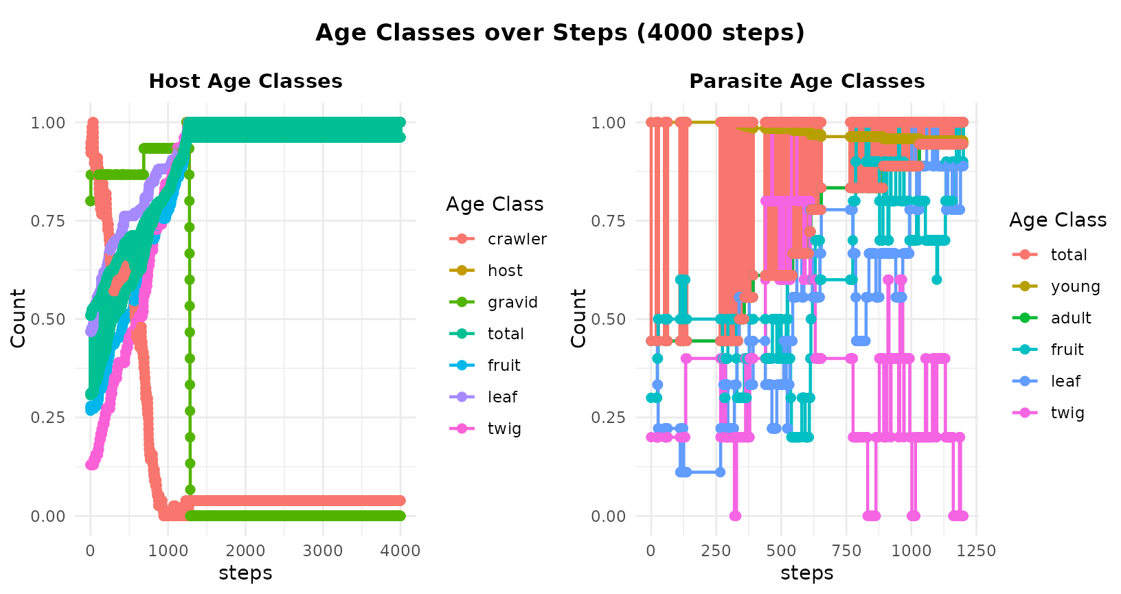

plot(simres, total = FALSE, normalize = FALSE, substrate = FALSE)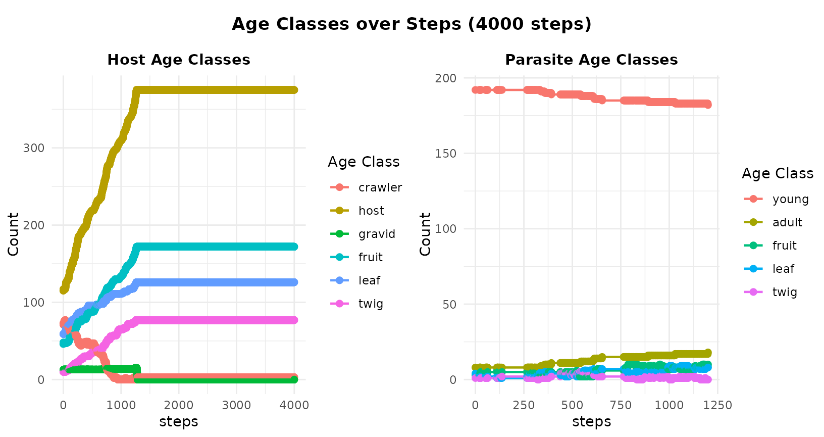

plot(simres, normalize = FALSE, substrate = FALSE)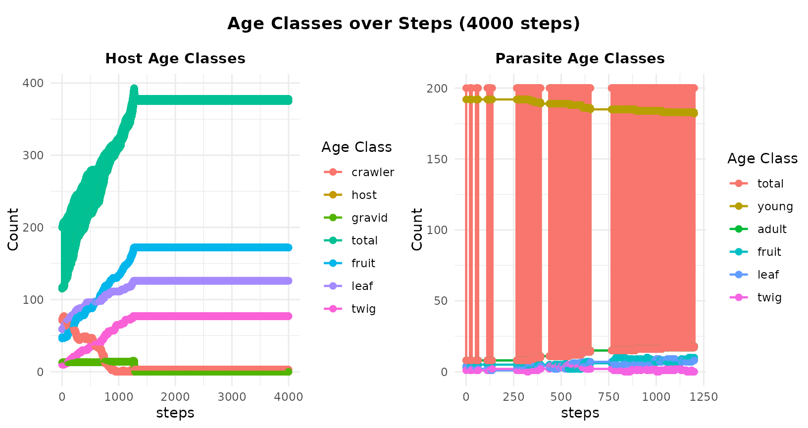

plot(simres, ageclass=FALSE)
#> [[1]]
#> Warning: Removed 1 row containing missing values or values outside the scale range
#> (`geom_text()`).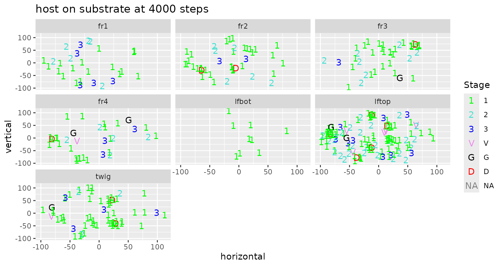

#> 
#> [[2]]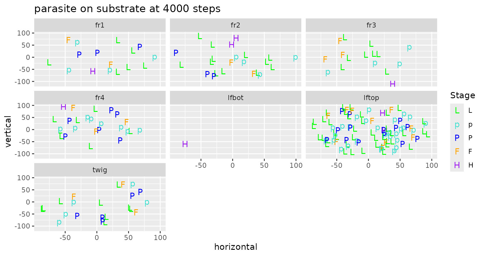

plot(simres, substrate = TRUE)
#> [[1]]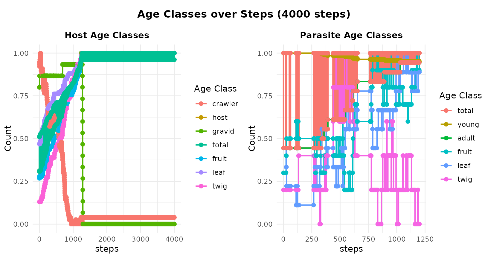

#> 
#> [[2]]
#> Warning: Removed 1 row containing missing values or values outside the scale range
#> (`geom_text()`).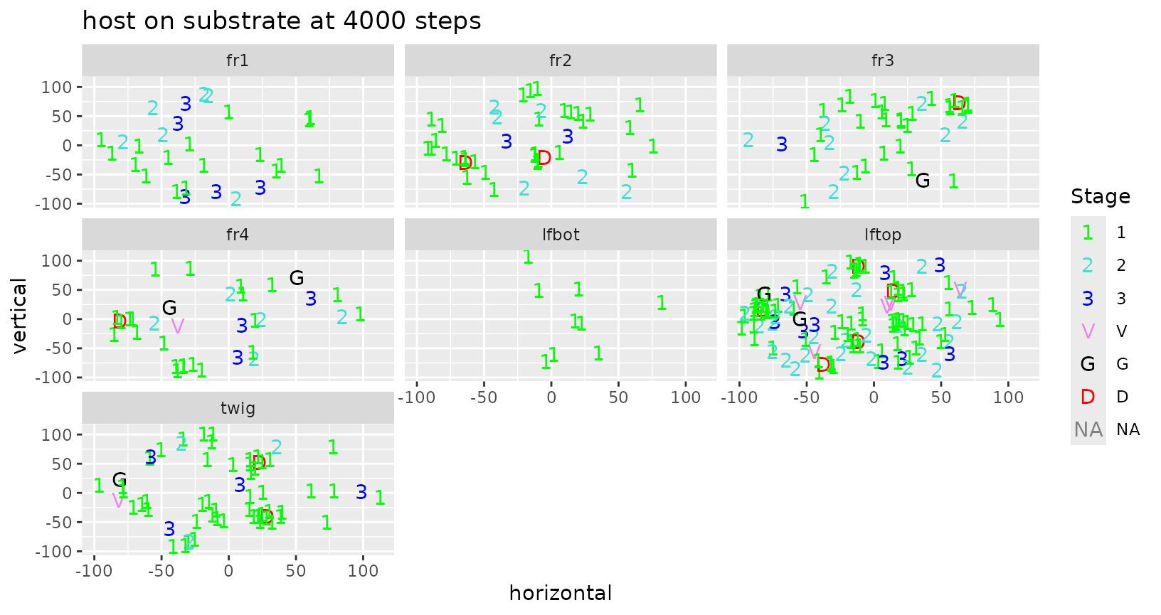

#> 
#> [[3]]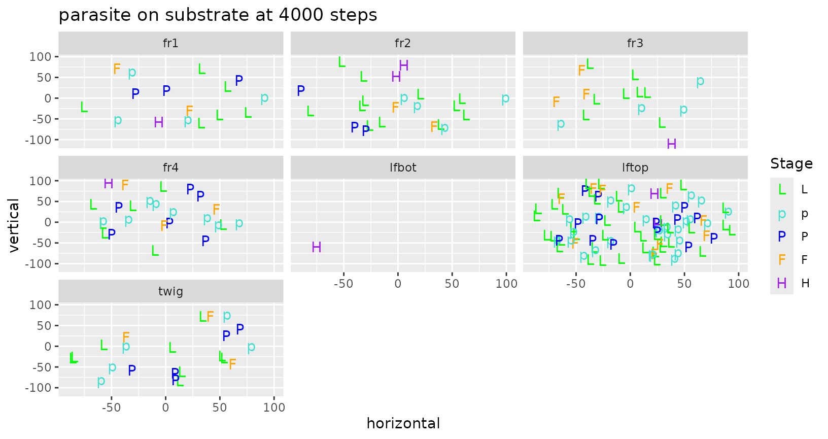

The object “mysim” has the initial populations and the organism and temperature structures. The object “simres” has the populations after running future.events (used to be step.future), along with summary information from the run.

I have also modularized the immediate, pending and future events. The functions

event.birth birth immediate event
event.attack    attack immediate event
event.death death pending event
event.future    generic future event

You can supply your own version of these if you don’t like mine. And you can add new ones by making appropriate changes in the “event” column of the future.host and future.parasite column. Adding a new kind of event, such as migrate means the routine now looks for a routine called “event.migrate”. Also, event.attack uses the type of parasite (endo,ecto) and the actual event (feed,ovip) to look for routines like event.ecto.feed to process attack details.

Multiple Simulation Runs

data(simdata)

summary(simdata)
#> 100 Runs of  4000 Steps for host=200, parasite=200
#> # A tibble: 10 × 8
#>    species  item        r central    lo    hi whisker.lo whisker.hi
#>    <chr>    <chr>   <dbl>   <dbl> <dbl> <dbl>      <dbl>      <dbl>
#>  1 host     crawler     0    69      62    79       36.5      104. 
#>  2 host     crawler   112     3.5     0    35      -52.5       87.5
#>  3 host     host        0   118     108   129       76.5      160. 
#>  4 host     host      112   286     245   334      112.       468. 
#>  5 host     gravid      0    14      10    18       -2         30  
#>  6 host     gravid    112    19       2    25      -32.5       59.5
#>  7 parasite young       0   190.    187   194      176.       204. 
#>  8 parasite young     116   180.    173   186      154.       206. 
#>  9 parasite adult       0     9.5     6    13       -4.5       23.5
#> 10 parasite adult     116    20.5    14    27       -5.5       46.5

ggplot_ewing_envelopes(simdata)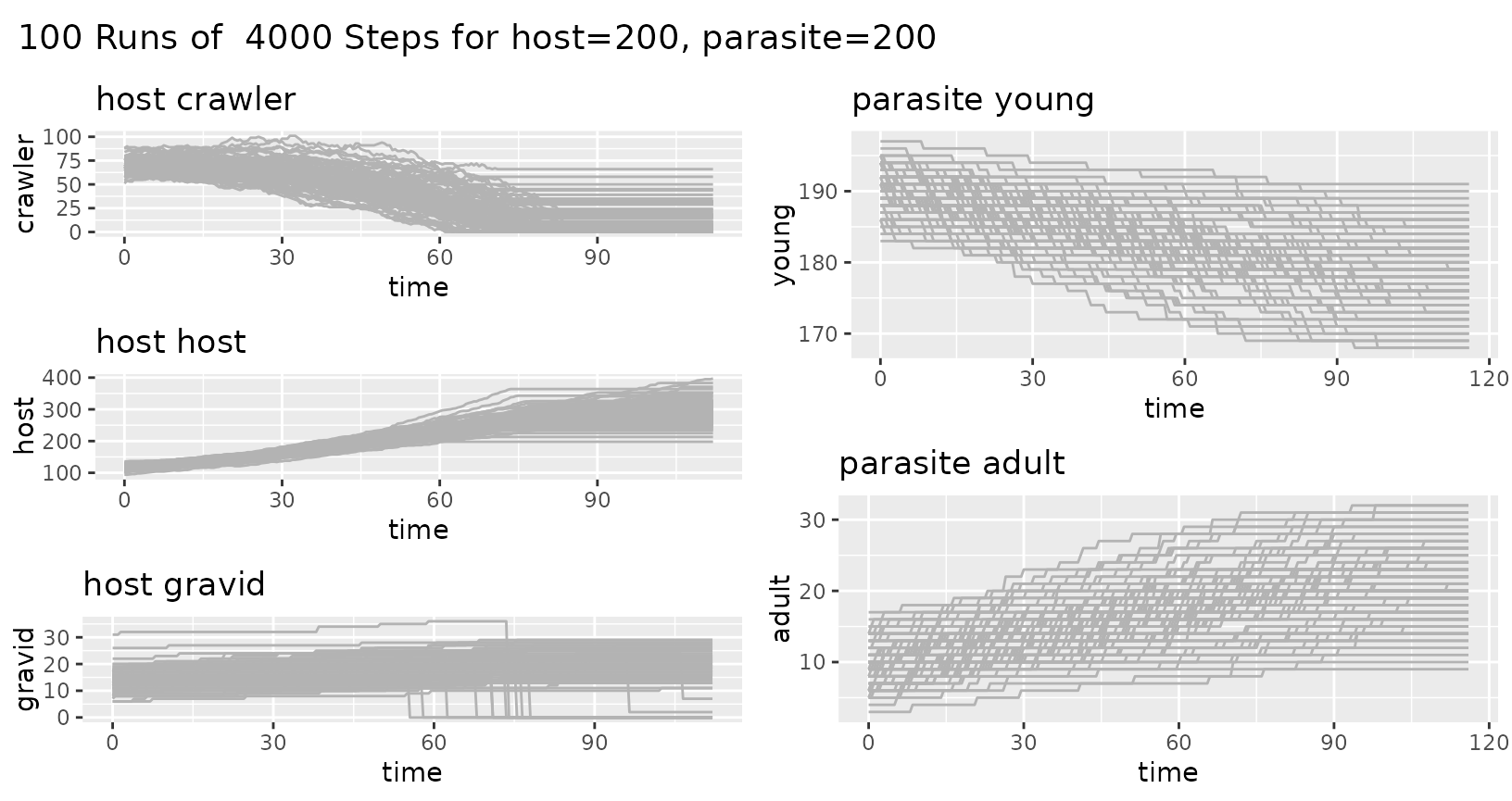

ggplot_ewing_envelopes(simdata, confidence = TRUE)
#> Warning: Removed 152 rows containing missing values or values outside the scale range
#> (`geom_ribbon()`).
#> Warning: Removed 125 rows containing missing values or values outside the scale range
#> (`geom_ribbon()`).
#> Warning: Removed 192 rows containing missing values or values outside the scale range
#> (`geom_ribbon()`).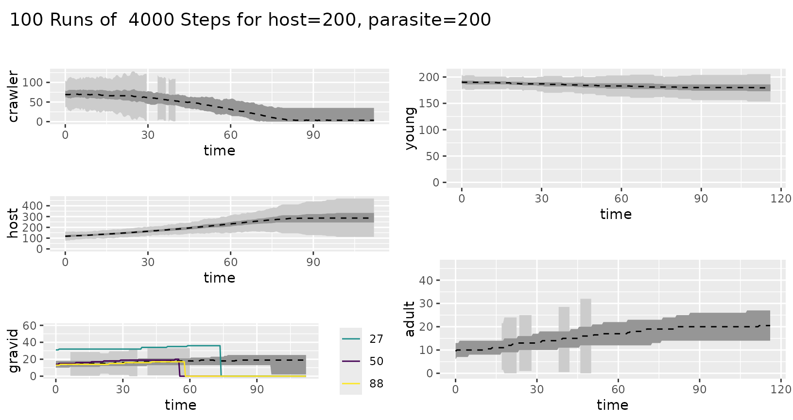

Other plots

ggplot_current(simres, "host")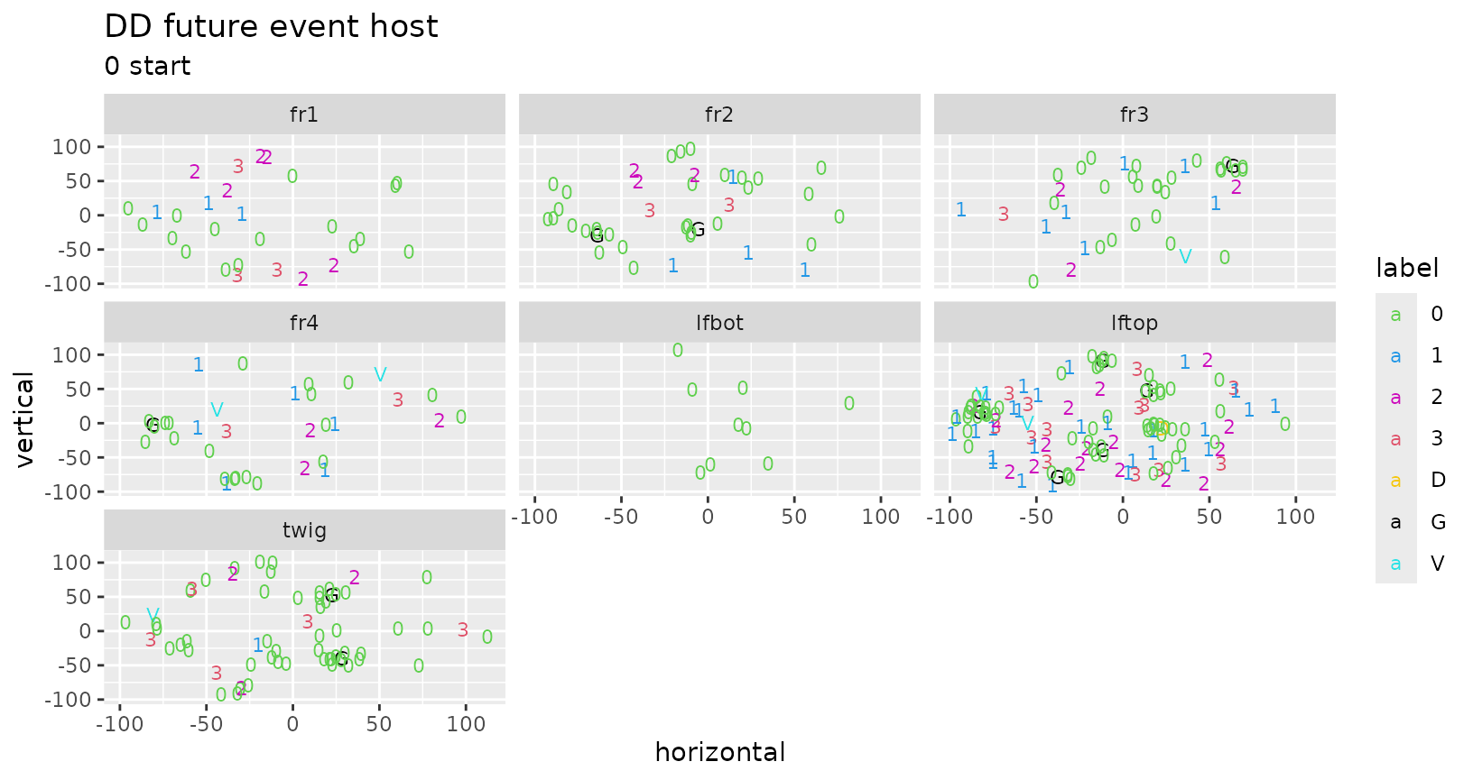

ggplot_current(simres, "parasite")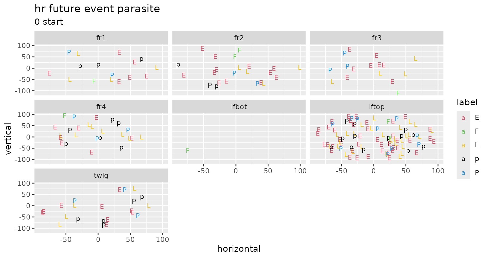

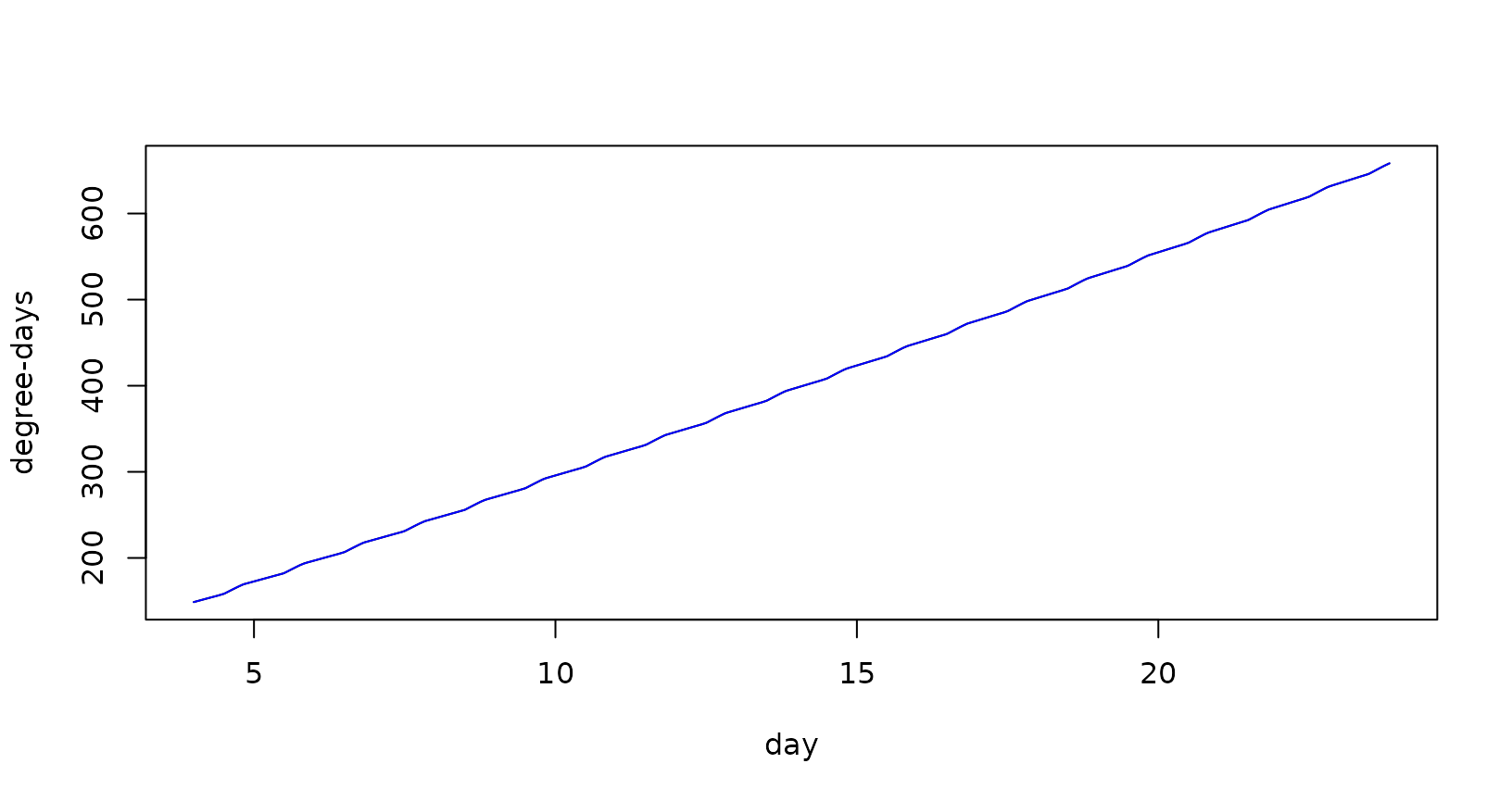
Plot to relate day to degree-day based on temperature regime.

temp.plot(simres)

Interactive

These plots show splines use graphics::locator() to adjust nodes.

The routines five.plot() and five.show() are two different versions of an interactive study of the 5-parameter relationship of time and mean value.

five.plot()

five.show()

interactive design plot for high and low temperatures. Uses graphics::locator().

temp.design(simres)

Inner workings of ewing simulation

Simulations are driven by flat files that declare the species, their relationships with each other and with the model substrate, and the details of scheduling future events for individuals. There are also files that specify the temperature regime, which is important if species respond to degree-day (DD) cues rather than temporal cues; this aspect is only briefly developed (see some plot ideas above) and will not be discussed further below. Here we use the default files in the data part of this package.

These simulations keep track of the current stage and next scheduled future event for every individual. That is, these simulations are individual-based rather than population-based. It is useful (such as for plots and other summaries) to collapse over individuals to get population trends, but impossible to reverse this without unrealistic assumptions. To that end, summary information at the population level (say by species life stages) are accumulated during the simulation, and later simplified for plots and tables.

This simulation is set up so that names of species, their stages, and subtrates are taken from the flat tables rather than being hardcoded. They are not limited to two species, although ultimately interactions are dyadic (two individuals) and monadic choices of future trajectories come down to competing risks for individuals.

Initialization

One begins a simulation by initializing all species. The organism.features table specifies multiple features of the simulated community. The units specify whether a species’ internal close is regulated by the hour (hr) or by degree-day (DD). The offspring is either a Poisson mean number (for a host species) or the name of the host species (for a parasite species). Similarly, attack is set to the host species for a parasite or NA if species is not a parasite. The parasite column specifies the type of parasite (ecto or endo; NA if not a parasite).

The deplete is the inverse of the depletion rate over time for individuals in species relative to time units that have passed. That is, the depleteion rate = (time lapse of event ) / deplete (leading of course to death unless the individual feeds. For species that are not parasites, the birth column has the stage when births occur (gravid for host).

Individuals in a species may move across a substrate. Which ageclass (subclass) of a species moves across the substrate? (host for host and adult for parasite; used for counting) and which stage of a species can actually move along the substrate?

Each species has a future event scheduling table (future.host and future.parasite). The init column specifies the relative weight of current stages for simulating the initial population.

Future events and competing risks

Each row of a future event scheduling table has possible future events from a current stage in the life of an individual of that species. The fid points to the row in this table corresponding to the future stage. The code uses numeric fid because it ends up in a vector of other numeric values. An individual in a species will progress from current to future stage when its event time is at the top of the event queue, unless some interaction leads to a change for that individual. The future event time is scheduled using the time entry. When an individual is at the top of the event queue, the future event time is scheduled using a spline interpolation with mean from the time value. If the species uses hours (hr), the spline is just a straight line, but if it uses DD the spline uses information from the temperature profile for the simulation (again, not discussed here yet).

Note that sometimes there are multiple rows with the same current value, which are competing risks. For instance future.host has competing risks from the current stage second.3 of becoming female or male, while future.parasite has competing risk from the current stage adult to feed or oviposit, with return lines from feed and ovip to adult. That is, an adult parasite might feed or oviposit, which have different health and population consequences: feeding prolongs life while ovipositing produces new offspring and depletes life.

All individuals have a current stage and are organized into an event queue, which is a triply-linked leftist tree, based on the scheduled time for their next future event. Each species has its own leftist tree, with the tops of those trees identifying the individuals with the closest (in time) next future event. Internal routine put.species, in conjuction with leftist.update, leftist.remove or leftist.birth, modify the leftist trees when there is an individual event update, death (remove) or birth(s), respectfully.

Plots and summaries

Plots used the plot character (pch), color (for stage) and ageclass (for summary grouping). The event column is useful for summary tables and plotting, and sometimes for other categorization (such as distinguishing birth and death from other types of future events).

Substrates and movement around triangular grid

This simulation system allows for individuals to be dispersed across a set of substrates and to move within and between substrate elements. Currently, each substrate is designed on a triangular coordinate system of interconnected triangles with diameter of 10 units (hardwired in internal routine event.move). Connectivity of substrate segments is determined by table substrate.substrate, while movement options for species are determined by species tables (substrate.host and substrate.parasite). substrate elements may have sides (1,2,3,4 for fruit, and top, bottom for leaf). Relative weights for movement are specified for initial position, chance of a parasite to find a host, and choice to move among substrate elements. The last columns of the substrate species tables give the relative weight of moving from the current substrate to one of the other substrates.

The triangular grid and approximations used herein capture most (~95%) of movement while simplifying calculations to max and min primarily rather than using quadratic calculation needed for a rectangular coordinate system (where the Pythagorean theorem rules).

Excel input data file

Users can supply and input data file to modify the simulation setup. In consists of the following sheets:

control sheet naming species, substrates, and key simulation parameters
- organism.features
future event sheets
- future.host, future.parasite (one per species; substitute name used in organism.features)
- host.parasite (one per each species interaction)
substrate movement sheets (currently only one substrate allowed)
- substrate.host, substrate.parasite (one per species; substitute name used in organism.features)
- substrate.substrate (connectivity of substrate components)
temperature sheets
- temperature.base, temperature.par

There are specific, fragile, constraints for naming of and within these sheets. Here are the “rules”:

organism names (first column or rownames of organism.features) must agree with the names for future event and substrate movement sheets
- default: host must match sheet names future.host and host.parasite
- default: parasite matches sheet names future.parasite and host.parasite
parasites are identified by several things
- entry ecto or endo in column parasite of organism.features (NA for non-parasites)
- entry host (substitute name of host) in column offspring and/or attack (NA for non-parasites; name is not currently checked to match name of a possible host)
- the word parasite (substitute name of parasite) must be in the rownames of the host.parasite (substitute names of host and parasite) sheet
non-parasites (such as hosts) are identified by several things
- birth column of organism.features needs valid current stage from non-parasite future event sheet
- default: gravid matches entry in current column of future.host sheet
- offspring column of organism.features has number (default: 20 for host)
- attack column of organism.features is empty (NA)
- empty (NA) in column parasite of organism.features (ecto or endo for parasites)
subclass column of organism.features must match valid ageclass of each species
- default: host matches ageclass entry in future.host
- default: adult matches ageclass entry in future.parasite
- smaller: grown matches ageclass entry in future.host
- smaller: forager matches ageclass entry in future.parasite
move column of organism.features must have valid current stage for each species
- default: crawler matches current entry in future.host
- default: adult matches current entry in future.parasite

Redscale thoughts

The fields are mostly self-explanatory. DD represents mean degree days to that future event. Thus the mean time to “virgin” from “third.3” is 560-465=95 DD. The next two fields concern the Aphytis parasite, comprising the relative risk of being killed by an Aphytis that is feeding or is laying eggs, respectively. There was no explicit information on feeding risk, so these are made up following Luck’s papers. The egg-laying risks are directly from the IPM pamphlet. The next two fields have the relative risks for the other two parasites. Then follows the gender (only females modeled here). The next field has the plotting symbol (pch), followed by the plotting color. The last and most important column is the life stage.

Scaling up

The beginning simulations use hundreds of individuals and thousands of simulation steps, as well as tens or hundreds of replicate simulations. Theoretically, it should be possible to scale simulations up to hundreds of thousands of individuals through some attention to loosely coupled systems and GPUs. At small population sizes, these simulations may shed new light on shortcomings of population-based simulations, but it is in large scale that they have the potential to provide useful insights for systems-level study.

It is useful to note that the simulation steps through events rather than time. Hence time is a function of events. Only in retrospect can the linear time sequence, and population numbers, be measured. Further, the relationship between steps and time is nonlinear, so that many steps may cover only a short time span, or a few steps may traverse much time. Further, different species may have a different relationship of steps to time. That is, the resolution for a species is set by the granularity of events and their mean time duration. The span of the simulation is determined by the number of allowed steps, and may result in different spans for different species, when taking into account the unrealized future events that remain in the community at the time of simulation stop.

03 August 2026